Singular Value Decomposition - SVD

Let us start from the centered parameter vectors (see Eq. 4 in the previous section):

(1)

This is a N by M matrix. Here N is the number of parameters describing each system or measured in each experiment. M is the number of experiments (or systems).

For any real rectangular matrix exists a factorization of the form

(2)

Here U is an N by K orthogonal matrix of the left singular vectors u_k, V is an M by K orthogonal matrix of the right singular vectors v_k, S is a K by K diagonal matrix of singular values s_k , and K is min(M, N). It is always possible to arrange the values in decreasing order:

(3)

The above factorization (2) is called the Singular Value Decomposition (SVD). The U and V matrices can always be expanded to square matrices. In this case S is a rectangular matrix with the non-zero elements s_k,l only for k = l.

Space of Parameters

The left singular vectors form the orthogonal basis in the N-dimensional space of parameters:

(4)

or in a matrix form

(5)

Here I is the identity (unit) matrix.

Any vector of the parameters from (1) can be presented as a linear combination (weighted sum) of these basis vectors:

 

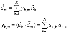
	(6a)
	(6b)

Space of Experiments

The right singular vectors form the orthogonal basis in the M-dimensional space of experiments (systems, measurements, samples):

(7)

The matrix of experiments (1) can be presented as a set of M-dimensional row vectors of experiments:

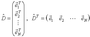
(8)

Any row of the matrix (1) can also be expressed as a linear combination of the v-vectors similar to (6).

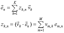
(9)

 

Principal Components

Equation (2) can be rewritten as

(10)

If the singular values s_k quickly decrease with k, then a small number of the above components is sufficient to explain most of the observed data. These components are called Principal Components both in the space of parameters and the space of systems.

In the case of two components, Eq. (6a) reduces to

(11)

It means that the m-th system is determined by two coordinates y_1,m and y_2,m along the axes u₁ and u₂ respectively. Graphically the m-th system is presented as a point on the (u₁, u₂) plane:

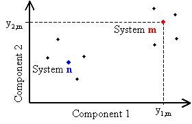
Fig.1. Principal component representation of systems

In the case of three principal components, a system is presented as a point in a three-dimensional space.

 

Relationship between the parameter bases

The initial parameter vectors can also be expressed  in the form (6) :

(12)

where the basis vectors p_n are

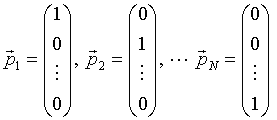
(13)

and also form an orthogonal basis in the space of parameters.

The matrix elements u_n,k in (6b) are the coordinates of the new basis vector u_k in the initial p-basis. The difference between the d-coordinates in the p-space and the y-coordinates in the u-space is more clearly seen in covariance matrices.

 

Covariance

The covariance matrix for parameters (1) is proportional to (see the previous section). Using (2) and (7) we have

(14)

Similarly, for the new coordinates  y_k,m we have

(15)

In Eq. (11)  is a square (K by K) diagonal matrix with the diagonal elements s_k² . It means that the combinations of the parameters parallel to the u-axes have zero covariances. In other words, they are mutually uncorrelated.

 

Principal component analysis

Principal components allow performing the following

1. Data compression or dimensionality reduction,
2. Noise filtering,
3. Correlation identification
4. Grouping of systems

To illustrate this, suppose that R < K principal components can reproduce the experiment within experimental errors.

1. It means that the data can be described by R*(N+M+1) values instead of the initial N*M values. 
2. The remaining  (K-R) components represent the noise and throwing them away effectively filters the data.
3. The combination of parameters corresponding to the largest singular values (i.e. proportional to the u-vectors) represent a strong internal connection.
4. Often visualizing the systems in 2D or 3D by plotting them in corresponding principal component subspaces reveals their separation to subclasses (see Fig. 1). 

 

This approach is implemented in a program called "Stat Analysis". This program is available in the Download section below.

 

Appendix. Reduced and full SVD

 For representation of a rectangular matrix in the SVD form (2) the reduced SVD is sufficient. The matrices have the following dimensions

Table 1.

Matrix	Dimensions
D	N x M
U	N x K
S	K x K
VT	K x M
V	M x K

where K = min(M, N). However in this case either U or V (depending on which one is rectangular) does not form a full basis in the corresponding space. It may cause problems in general algebraic analysis. In particular, one of these matrices does not have the inverse matrix.

This can be easily resolved by extending the corresponding matrices so that both U and V are square and form a full basis. In this case the dimensions are

Table 2.

Matrix	Dimensions
D	N x M
U	N x N
S	N x M
VT	M x M
V	M x M

Some variants of the SVD algorithm can perform a full decomposition at once.

Example

Let us consider the case when the number of experiments is greater than the number of parameters, M > N ( K = N ). The reduced SVD can be illustrated in the Fig. 2.

Fig. 2. Reduced SVD

The number of v-vectors is less than their dimension:

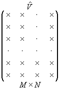
N < M

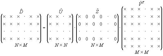
 Below is the extension of the above decomposition to the full SVD.

 

Fig. 3. Full SVD

 Note, that now S has extra M - N zero columns.

Download

1. Program "Stat Analysis".

References

1. Singular value decomposition.