Introduction

If some unit of measure can be applied directly, then this type of measurement is called direct measurement. Example:

Human eyes determine the distance from the different angles of the each eye line of sight:

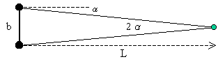
This is an example of indirect measurement. The determination of the distance L requires additional processing:

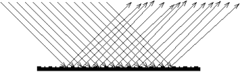
Very often we measure not what we need but what we can, and try to estimate the quantity of interest. For example, we can measure the properties of light reflected by a surface and estimate the surface roughness:

We also prefer to detect a harmless radio signal in magnetic resonance imaging rather than really slice a body:

The obvious areas of indirect measurements are very small or very large or remote objects. In general, this is the measurement of the objects that are inaccessible for direct measurements.

Measurements scheme

This is a schematic presentation of the process of measurement:

1.  Input signal is any field interacting with the object (electromagnetic irradiation, heat, light, radiation, electric potential, acoustic and seismic waves, chemical and nuclear reactions).
2. Object is any part of the measuring system 
3. Object response is the transformation of input signal (reflection, deflection, reemission, frequency and phase change, electric current variation, chemical transformations) 
4. Accuracy and interval of measurements are important characteristics of signal detection.
5. Processing is the evaluation (retrieving) the properties of the system (objects). Accuracy and resolution are the most important characteristics of the processing.

Linear systems

Usually the systems are assumed to be "Linear". It means that the total signal (response) from the system is the sum of the signals from its subsystems. In particular, the signal from the subsystems with the same parameters is proportional to the number of such subsystems (Linear dependence on the number). 

System parameters and Measured parameters

Mathematically the measured signal from a linear system can be presented in the following form

Here is the number of x-th subsystems, is the signal from this subsystem as a function of the scanning parameter y (e.g. the dependence of intensity in the receiving coil on input pulse duration).

The system parameters here are denoted as x. For example, it can be a particle radius in air pollution control measurements or three coordinates (a vector) of the point in human body in MRI.

Here for simplicity we restrict ourselves with one scanning parameter and one system parameter (in other words, both parameters are scalar).

Integral Form

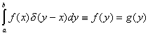
When x is a continuous parameter then the above sum is replaced with the following integral:

Actually, this is an equation with unknown function  f and the right-hand side function g. This equation is known as the Fredholm integral equation of the first kind, and is called the kernel of this equation. The kernel is a mathematical description of the method of measurement. The interval of system parameter variation [a, b] and the measurement interval [c, d] are the part of the measurement description as well.

Naïve solution

For the first sight, the above equations can be easy resolved. If the signals from each subsystem  are known in the set of discrete points y_m, then we can always adjust the linear parameters so that the combined signal fits the measured signal . Actually, this is a set of linear equations:

Here is the matrix of the above system, is the unknown vector, is the r.h.s. vector. The integral equation is just a very big set of linear equations. 

However the computational practice shows that the solution of this system is unstable and very sensitive to experimental errors. 

 

Ill posed problems

Unfortunately, in general, the above equations belong to the case of so-called ill posed or ill stated problems. These problems have at least one of the following features:

• The solution does not exist for arbitrary r.h.s.
• The solution is not unique
• There is no continuous dependence of the solution on the r.h.s. 

The Fredholm integral equation of the first kind can have all of the above features. Of course, it depends on the kernel (and the intervals [a, b] and [c, d]). 

 

Kernel functions

The best kernel is -function: . The -function is the extreme case of the very narrow large peak so that

 

The integral equation reduces to 

In fact, this is a mathematical model of direct measurements.


Delta-function approximation
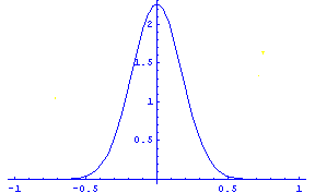
The -function can be approximated by a rectangular with the width w and the height 1/w so that . Another popular approximation is the Gaussian function:

This is its graphical representation:

Gaussian peak G(x)	Gaussian kernel G(y-x)

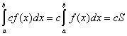
The worst kernel is a constant, K(y,x) = c :

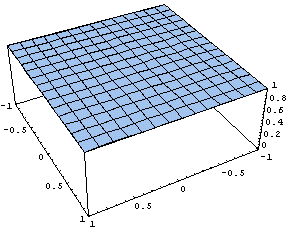
The constant kernel K(y,x) = 1

It allows determination only of the area S under the curve f(x):

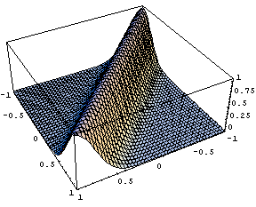
Model kernel

The kernels corresponding to real measurements are far from the both extremes. They are not necessarily symmetrical because they connect the parameters of different nature.

Let us consider the measurements which mathematical model has the following simple kernel:

This is a very broad peak:

The model kernel

It can be directly shown that for any f(x) 

where

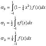
Some conclusions

• It means that the left-hand side of the integral equation is always a polynomial of the degree not more than 2. Different functions f(x) can only change the values of the factors .
• If the right-hand side of the equation is not a second-degree polynomial than the solution does not exist.
• If both f(x) and g(x) are the polynomials of the second degree than the solution is unique:
  for we have

  

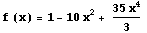
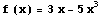
• Without the additional information (as we used above the assumption about the degrees) the solution is not unique. The two examples of the functions that give zero contribution to the signal g(y) are presented below:

   

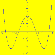
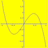
Incomplete measurements

The zero contribution means that such components of the function cannot be detected and, consequently, cannot be restored even for absolutely precise measurement. In other words, this is incomplete measurement and for the extraction of the "lost" information we need some additional measurements. This is quite natural: it is difficult to imagine some universal experiment, which measures everything.