Error: Estimation | Amplification | Propagation

Introduction

In the previous section we discussed a basic error estimation. Here we consider the propagation and amplification of errors during data processing. The simplest procedure is the solution of a system of linear equations.

Let us start with the following example:

(1a)

The inverse system is

(2a)

Obviously this is also a linear system.

Numerical experiments

Experiment 1. Compare the solution for  b₁ = 1 and b₂ = -1 with the solution for the right hand side with 1% noise.

b1	b2	x1	e1	x2	e2
1.0	-1.0	40.0		-20.0
1.01	-1.01	40.4	1 %	-20.2	1 %
1.01	-0.99	40.002	0.005%	-19.996	0.02%

Here e_i are the relative errors for the r. h. s. The accuracy of the solutions is also 1% or less.

Experiment 2. Compare the solution for  b₁ = 1 and b₂ = 1 with the solution for the r. h. s. with 1% noise.

b1	b2	x1	err1	x2	err2
1.0	1.0	0.2		0.4
1.01	1.01	0.202	1 %	0.404	1 %
1.01	0.99	0.6	300 %	0.2	50%

The result speaks for itself: a simple linear transformation can cause a catastrophic increase of an error.

Analysis

Assuming that the errors for b₁and b₂ are uncorrelated with the standard deviation σ, we get from (2) (see the appendix for details)

var(x1) = 800.02 σ2
var(x2) =  200.08 σ2	(3)
cov(x1, x2) = -399.96 σ2

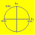
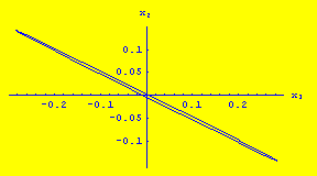
The errors for x are not only much larger but also are strongly correlated. This can be represented graphically. Two independent errors of the magnitude 0.01 form a circle in the  b₁, b₂ plane 

The corresponding solution errors form the following elongated ellipse in the  x₁, x₂ plane

Algebraic approach

Equations (1a) and (2a) can be rewritten as

	(1b)
	(2b)

Using the singular value decomposition (SVD) the matrices can be presented in the following form

(4)

and

(5)

where

(6)

 and

(7)

Any vector in the x-space can be presented as a linear combination of the vectors v₁ and v₂:

(8)

Similarly any vector in the b-space can be expressed in terms of u₁ and u₂:

(9)

Eq. (5) can be interpreted in the following way. The first term transforms the u₁ component of b into the v₁ component of x, and is the transformation factor. The second term transforms the u₂ component of b into the v₂ component of x. However, the transformation factor in this case is 100 times larger. This explains noise amplification.

Filtering

The components corresponding to large noise amplification cause instability in the solution of linear systems. The filters based on the SVD can improve stability without essential loss of accuracy.

Appendix

Extended variant of Eq. (3).

var(x1) = 404.01 var(b1) - 799.98 cov(b1, b2) + 396.01 var(b2)
var(x2) =  96.04 var(b1) - 199.92 cov(b1, b2) + 104.04 var(b2)	(1)
cov(x1, x2) = -196.98 var(b1) + 400.04 cov(b1, b2) + 202.98 var(b2)

Error: Estimation | Amplification | Propagation

References

1. Singular value decomposition (SVD).
2. Linear algebra: a summary of vector and matrix operations is available here.